The resolving power of optics

You are here: Nature Science Photography – Visual acuity – Image sharpness II

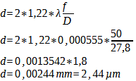
As we have already discussed in detail in the section „Imaging Sharpness I: Optics, Geometric Sharpness and Depth of Field / Circle of confusion and Diffraction Disks – Not Every Aperture Is a Good Aperture„, the imaging performance of an optical system is limited by the aberration on the side of the large apertures and the diffraction on the side of the small apertures. Everything that is stated there applies 1:1 also to the resolving power. In terms of diffraction, we can add that within the diffraction pattern, the width of the airy disk is used to determine the theoretical maximum resolving power of an optical system: It corresponds to the diameter of the first dark ring. For a 50 mm objective and aperture 1.8, we get:

Calculation 29

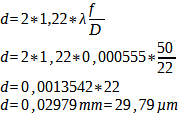
For the same 50 mm lens and aperture 22, the value increases to:

Calculation 30

Practically, as explained in the previous section, the MTF takes into account all factors when determining resolution. As previously explained, we may encounter MTF diagrams in the optics‘ data sheets. They can, but they don’t have to. Because strictly speaking, the contrast transfer function, as we have come to know it up to this point, defines the resolving power only for a single point in the image field. But because sharpness and resolving power of an optic are highest in the center and lowest at the edge, we actually need a separate MTF for every single point. For this reason, there exists an alternative representation that provides the MTF for a given spatial frequency as a function of distance from the image’s center.

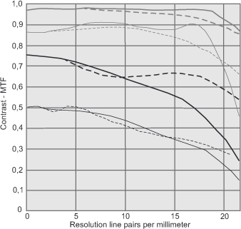
Figure 40 (MTF diagram of an average 35 mm lens)

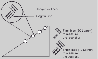
shows this using the Canon 1.4/50 mm lens as an example. This diagram has values between 0 and 1 on its vertical axis, which are shorthand for 0% and 100%. So 0.1 means 10% contrast, 0.5 equals 50% contrast, and 1 equals 100% contrast. The horizontal axis is divided into millimeters and indicates the distance from the center of the image (0) to the edge (20). Since a 35 mm image has a nominal width of 35 mm, this second point is at the edge of the image. The higher a point is in the diagram, the greater its contrast, and the further to the right it is located, the further it is from the center of the image. In addition, the figure shows black and gray, thick and thin, and solid and dashed lines, for a total of eight different line types. The thick lines represent the measurement results for the low resolution of 10 Lp/mm, the thin lines are those for the higher resolution of 30 Lp/mm. The black lines indicate the measurement results with the aperture open; the gray lines are those with the aperture stopped down to f/8. Last but not least, we have the solid lines showing the results for tangential lines and the dashed lines indicating those for sagittal lines. Figure 41 (Sagittal and tangential lines) illustrates these two types of lines.

Sagittal lines are those that run parallel to a diagonal line through the center of the image. Tangential lines run at a 90° angle to this diagonal.

In order to correctly interpret an MTF diagram in the form mentioned, we should remember a few rules:

• The higher the thick lines (10 Lp/mm) are in the diagram, the higher is the contrast reproduction capability of the lens. Lenses with this line type above 0.8 can be called excellent. If it is above 0.6, they are considered satisfactory. Any lower than this should not be considered.
• The higher the thin lines (30 Lp/mm) are in the diagram, the higher is the resolving power of the lens and thus the perceived sharpness of its image.
• The closer together the black and gray lines (open aperture and f/8, respectively) are, the better the imaging performance of the lens at open aperture. This comes in handy in the low brightness of available light situations.
• The closer the solid and dashed lines are to each other, the more pleasing is the image of those areas of the image that are actually out of focus. This is described by the Japanese word bokeh.

Finally, we should note that the contrast transfer function does not provide a comprehensive understanding of a lens’s characteristics. After all, important variables such as vignetting, linear distortion or susceptibility to flare are not indicated in it. Nevertheless, the MTF curve is a well-suited tool for assessing the resolving power of an optical system. It’s crucial to understand that the MTF curve should only be compared between lenses of the same focal length for accurate results. Comparing the MTF of a telephoto lens with that of a wide-angle lens will not yield meaningful results, as the construction of long focal lengths fundamentally outperforms that of short ones. Furthermore, comparing MTF diagrams from different manufacturers is often problematic. Some manufacturers give diagrams based on theoretical calculations, while other companies publish real measurement results. Therefore, the MTF comparison for lenses of one series is possible and helpful; the one for optics of different manufacturers may not be. So be sure to find out exactly where the data base comes from. Of course, this section applies equally to both capture lenses and enlarging optics.

Next The resolving power of analog image carriers

Main Visual acuity

Previous The contrast transfer function (MTF) – The central element for determining resolving power

If you found this post useful and want to support the continuation of my writing without intrusive advertising, please consider supporting. Your assistance goes towards helping make the content on this website even better. If you’d like to make a one-time ‘tip’ and buy me a coffee, I have a Ko-Fi page. Your support means a lot. Thank you!