The resolving power of digital image carriers

You are here: Nature Science Photography – Visual acuity – Image sharpness II

Just as with silver film, the size and spacing of the light-sensitive elements play the fundamental role in the spatial resolving power of digital image sensors. The Nyquist-Shannon sampling theorem
determines the structure size that a sensor can resolve with a given pixel size and number. The theorem states that we must sample a continuous band-limited signal with a minimum frequency fMin of 0 Hz and a maximum frequency fMax with a frequency >= 2*fMax. This allows us to reconstruct the original signal from the resulting discrete-time signal without information loss (but with infinite effort) or approximate it (with finite effort) with arbitrary accuracy:

Formula 29

Applied to our consideration, the theorem means that the maximum usable resolution in pixels or lines per unit length (maximum frequency) corresponds to half the number of pixels in each of the two dimensions of the sensor. In the case of a Canon EOS-1Ds Mark II with a horizontal pixel count of 4992 and a pixel pitch of 7.2 µm, the formula tells us that this camera has;

Calculation 31

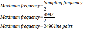
2496 line pairs in this axis and structures can be resolved up to a distance of 14.4 µm from each other (for two structures to be resolved as separate, they must be at least two pixels apart. Therefore 7.2 µm*2 = 14.4 µm). If we divide the 2496 line pairs by the width of the sensor (36 mm), we get the number of line pairs per millimeter. This frequency, also known as the Nyquist frequency, signifies the maximum spatial frequency at which the sensor can effectively capture real information.

Calculation 32

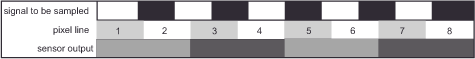
If the subject has structures that are close to or even above the Nyquist frequency, the image will have artifacts that the real scene did not contain due to the sampling frequency being too low for them. We refer to these artificial low-frequency signals as aliasing, which manifest as color fringes (moirés) in periodically repeating patterns and as jagged diagonal lines (jaggies) in non-repeating patterns. On television, the effect can sometimes be observed when the presenter wears a jacket in a very fine herringbone pattern. To avoid them, the combination of sensor and optic should ideally show no reaction (MTF = 0) above the Nyquist frequency. Unfortunately, this is not practically achievable, so we must equip the sensors with an anti-aliasing filter, also known as a low-pass filter, to prevent unwanted artifacts from appearing in the images. This is a vapor-deposited layer that absorbs light with wavelengths below the pixel pitch. It is kept as thin as possible to prevent additional disturbing effects, but overall, depending on the camera, it leads to a resolution reduction of up to 40% and a softer image that has to be improved again by subsequent sharpening. Only with particularly compact digital cameras (point-and-shoot) with pixel pitches of less than 4 µm is the attenuating modulation transfer function of the lens sufficient to prevent aliasing.

To put the whole theory in perspective, it is important to realize that the original signal is never clearly delimited, and there is no single meaning of analog reconstruction – printers, imagesetters and monitors are, after all, very different from each other. For these reasons, the original signal can never be reconstructed with true accuracy, and compromises between true resolution and aliasing are inevitable.

If you have thought along well up to this point, you might now object that the sampling theorem should actually also be applied to the silver film, but that I have neglected to do so in the relevant section. At first glance, this may seem plausible, but there are several compelling arguments against it. A conventional image sensor arranges its pixels in an absolutely regular and overlap-free manner, with all pixels having the same size. Not so with silver film. In this case, the silver particles are not uniformly distributed within the photographic layer, but rather, they are arranged more or less randomly and exhibit varying sizes. Moreover, the layer contains more than one silver halide crystal, further enhancing the randomness of the arrangement. Without geometric regularity, however, there is no mathematical calculability, and so Nyquist does not apply here. So the analog material works quite differently than the electronic image sensors, and we cannot directly compare the „film pixels“ with the digital pixels. The only practical way to compare the two is to look at the final results.

So far the theory. In order to practically achieve the number of line pairs calculated with it, it is of course necessary that the lines always fall exactly on separate pixels, and therefore the word „theoretical“ is especially important in this context. For realistically, it is extraordinarily foolhardy to assume that the structures of our subjects will do us the favor of arranging themselves so regularly. In the wild, we rather have to reckon with fine details slipping between two pixels, and if that happens, our just calculated theoretical measure is ruined. Of course, this practical behavior has a name. It is called the Kell factor after its discoverer, the TV engineer Raymond D. Kell, and is in the order of 70% to 80%. The Kell factor states that a system with a sampling rate of x can resolve 0.7*x lines in a given direction (horizontal or vertical). Attention, danger of confusion: The Nyquist theorem always pertains to line pairs, while the Kell factor pertains to individual lines. If you want to compare both, you must either multiply Nyquist by two or divide Kell by two.

We can verify the realistic nature of the Kell factor using a practical example. In their review of the Canon EOS-1Ds Mark II (effective pixels 4992 x 3328), the folks at dpreview.com give a measured resolving power of 2800 lines horizontally and 2400 lines vertically. These 2400 lines vertically correspond to 72% of the 3328 pixels in this plane. If you now object that the 2800 lines in the horizontal plane correspond to only 56% of the pixels there, please note that they have calibrated their resolution test with respect to the number of lines per image height. So the numbers are comparable without having to consider the aspect ratio. Therefore, to determine the value for the lines per image width, multiply the given number by the aspect ratio, which is 3:2 = 1.5, resulting in 2800*1.5 = 4200 lines or 84 %. This value aligns with Kell’s predicted spectrum. We can go one step further. If you divide the values calculated with the Kell factor by two to make line pairs, the results for the horizontal and the vertical roughly correspond to 2/3 of the maximum values predicted by Nyquist. You can remember the value 2/3, because if the sensor has an anti-aliasing filter, it will lock at about this value.

Material on the contrast transfer function (MTF) of real digital sensors cannot be found from the manufacturers, but can be calculated approximately with mathematical models. A function that has proven itself in this respect is:

Formula 30

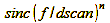
where dscan is the sensor resolution in pixels/mm. Norman Koren (http://www.normankoren.com) has compared the findings of the Imaging Technology Research Group of the University of Westminster/UK (1,2), which led to this function, with the results presented by Don Williams of Eastman Kodak in (3). He concludes that different values for n can simulate Bayer-pattern sensors with and without anti-aliasing filters and chips of the Foveon type.

• The MTF of Bayer pattern sensors with anti-aliasing filter is approximately equal to the function sinc(f/dscan)³
• The MTF of Bayer pattern sensors without anti-aliasing filter (especially point-and-shoot cameras with pixel sizes <= 4µm) approximates the function sinc(f/dscan)²
• The MTF of a Foveon X3 sensor, which due to its mode of operation does not require interpolation and also does not have an anti-aliasing filter, corresponds approximately to the function sinc(f/dscan)^1.5

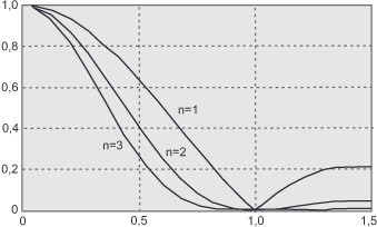
Figure 45 (Simulated MTF curves) shows the MTF curves calculated according to this pattern. The three curves clearly show how negatively interpolation and anti-aliasing filters affect contrast and resolving power. The Foveon sensor, which operates without these two obstacles, outperforms the others in both respects (n = 1.5), placing it between the first and second curves from the right. The curve of the Bayer pattern sensor, which does not have an anti-aliasing filter, follows at a significant distance, particularly in contrast (n = 2).

The resolution behavior of colored structures

Up to this point, everything relates to grid patterns of black and white structures, and therefore applies to the spatial resolution of structures that differ in terms of their brightness. Since we saw at the beginning that our visual system shows a different resolution behavior for colored templates than for black and white ones due to the structure of its information processing (where-path, what-path), we should also consider the electronic image carriers in this respect.

Bayer pattern sensors have twice as many green pixels as red and blue ones because our visual system is most sensitive to the medium-wave range of the spectrum.

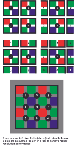
Bayer pattern sensors generate color through the demosaicing process. This is the name given to the process in which the primary color filter pattern (Color Filter Array, CFA) is translated into a finished image with full color information in each pixel. Since each sensor point only provides information about one area of ​​the spectrum (short wave/blue, medium wave/green, long wave/red), the demosaicing algorithm has to interpolate the two missing pieces of data, or „guess“ them, so to speak. To do this, it relies on the neighboring pixel values ​​and makes something known as an educated guess. The individual pixels are grouped into fields measuring 2×2 elements and calculated with respect to their spatial and/or chromatic relationships. The mathematics behind this varies from manufacturer to manufacturer and is a closely guarded secret, because it is a major factor in determining image quality. In addition, new algorithms are constantly being published. The currently highest quality ones also include the stored knowledge about a large number of natural scenes in their calculations, so they are adaptive with respect to the image content.

As far as the resolution for colored structures is concerned, it should be noted that it drops to half the brightness value in the horizontal and vertical direction if the camera stubbornly places these 2×2 element fields next to each other and adds them up to a new pixel value (Figure 46). This would be the worst case. To achieve a higher value, overlapping areas are used (Figure 47). In this way, the resolution ends up somewhere between the full and half value. But that’s not a bad thing, because our resolution is six times worse in this respect.

Cameras with Foveon sensors (mainly those from the manufacturer Sigma, to which Foveon Inc. belongs) do not have such a gradient. These image carriers integrate three layers on top of each other for red (long wave, top), green (medium wave, middle) and blue (short wave, bottom). Thanks to this more complex architecture, which takes advantage of the fact that light of different wavelength ranges penetrates the silicon to different depths, they provide the full color information, i.e. resolution, at each pixel. What looks like an advantage at first glance is not one, because color resolution on the same scale as brightness resolution is wasted thanks to our physiological conditions – we simply cannot perceive it. Only if you use special test panels with color combinations that have the same brightness (i.e. are isoluminant) does Foveon technology have an advantage over the Bayer pattern. But in these cases we would have the same difficulty recognizing the test patterns and outside of laboratories we only encounter subjects without changes in brightness extremely rarely.

Now and again you hear and read the assumption that the brightness resolution of Bayer pattern sensors is only half as large as that of the monochrome Foveon layers because of the block formation of 2×2 pixels required for demosaicing or because supposedly only the „green pixels“ are used for the brightness signal. But that is wrong, because since the spectral characteristics of the blue, green and red filters are known, the brightness value (Y) can and is determined as a weighted average for each individual pixel according to the ISO specification Y=0.2125*Red+0.7154*Green+0.0721*Blue.

But what if, and this is another common objection, the subject is, for example, purely green? In this case, the values ​​of the blue and red pixels would have to be zero and thus useless for calculating the brightness. But this assumption is also wrong, because it assumes that brightness and color in each pixel are completely independent of each other. But they are not, because we have seen up to this point that the RGB value of each pixel is based on the size measured at each sensor point plus the size of the neighboring sensor points. The camera can make this calculation correctly for all image details that are no finer than 0.25 line pairs/pixel (because a maximum of 2×2=4 pixels are needed to resolve a full cycle in color). Problems can only arise in the highest octave of the spatial frequencies, which includes the finest image details. There, the algorithms can falsely create color based on some black and white patterns and, conversely, black and white information on color structures. But that is relatively rarely the case, because it requires that the spatial frequency corresponds almost exactly to the Nyquist frequency. Nevertheless, the errors are very disturbing when they occur.
Bayer pattern sensors therefore provide enough information to correctly display all coarser patterns, regardless of whether they are black and white or color, and in terms of brightness resolution, they do not give up any ground compared to monochrome (Foveon) sensors. Otherwise, the directly measured resolution values ​​for black and white grid patterns presented above, which are at the limit of what is theoretically possible, would not be explained.

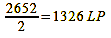
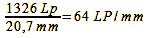
In theory, the Foveon design only offers advantages in a few exceptional cases. In practice, it has so far been inferior to the Bayer pattern in every case in terms of resolution. This is mainly because Sigma has not yet managed to bring Foveon sensors with competitive pixel counts onto the market: the SD15 (sensor size 20.7×13.8 mm) has an effective 2852×1768 pixels, a Canon EOS 500D has 4752×3168 pixels with a comparable sensor size. This is probably primarily due to cost reasons. The large number of Bayer-pattern sensors produced allows a lower unit price than the Foveon model, and so in the first case you get more pixels for the same money, i.e. a higher resolution. So that their cameras do not perform significantly worse in the various tests than comparable Bayer-pattern cameras at first glance, Sigma specifies the resolution in line pairs per pixel and not, as is generally the case for better comparability, in line pairs per image height. In addition, the anti-aliasing filter is still omitted, which leads to moirés, which are often mistakenly interpreted as real resolution. The fact is, however, that the Nyquist-Shannon sampling theorem and the Kell factor apply to Foveon sensors just as much as to those with a Bayer pattern. In order to keep the comparison fair, the different pixel numbers and sensor sizes must also be taken into account (format factor to compare the Sigma SD15 with the Canon EOS 500D = 1.08). This gives the Canon EOS 500D a Nyquist frequency of:

Calculation 32a

Calculation 32b

The calculations speak for themselves and there is no getting around the bare numbers. But that does not mean that the Foveon technology is fundamentally bad, quite the opposite. With almost the same number of pixels and an anti-aliasing filter, cameras with such image capturers would be the ultimate solution, because they would not suffer from the rare but annoying, structurally-related color moirés of the Bayer pattern sensors. Both systems therefore (still) have significant disadvantages and every photographer has to judge which he is willing to accept based on the image results.

Smaller pixels = higher resolution?

Now you could simply demand that the pixels be made smaller in order to increase the resolving power. Unfortunately, I have to disappoint you on this point, just as I did with silver film. Partly for the same reasons, partly for different ones, because since we are dealing with electronic components at this point, new factors come into play that are not apparent at first glance. Firstly, the issues of sensitivity and contrast present in analog film resurface. Small pixels are less sensitive than larger ones and can digest a smaller contrast range due to the smaller overall size of the sensor. In both respects, pixels smaller than 4 µm perform particularly poorly. An electronic specialty is noise, the unwanted electrical activity of all electronic components that masks the usable signal. To work with the desired useful signal, we must overcome this obstacle. To separate the two, the signal-to-noise ratio (SNR) is defined as the ratio of the average power of the useful signal from the signal source to the average noise power of the noise signal from the same signal source. We can distinguish the signal from the noise as it rises from this value. Large pixels naturally collect a lot of light, produce a strong signal, and thus provide a good signal-to-noise ratio. Small pixels, on the other hand, collect less light, produce a weaker signal, and provide a comparatively poorer signal-to-noise ratio. Noise is thus more present in their output signal, and if you’ve ever compared images taken at ISO 400 with a compact digital camera (which typically has small sensors and small pixels) and a digital SLR (which typically has large sensors and large pixels), you can practically understand this. The exact relationship between pixel size and noise is not easy to pin down, as there are several mechanisms at work here that vary in strength. For these reasons, and due to cost – a large sensor with large pixels costs more because their yield in production is lower – the pixel size between 6 and 9 µm has emerged as almost optimal. Below this are the compact digital cameras, which offer sensors with diagonals between 5 mm and 11 mm on a pixel size of 3 to 4 µm or less.

Next The resolving power of digital output devices

Main Visual acuity

Previous The resolving power of analog image carriers

If you found this post useful and want to support the continuation of my writing without intrusive advertising, please consider supporting. Your assistance goes towards helping make the content on this website even better. If you’d like to make a one-time ‘tip’ and buy me a coffee, I have a Ko-Fi page. Your support means a lot. Thank you!